Moving Mountains: 2- to 3-Dimensional Topographic Models
- Joelle McDonald

- Apr 20, 2025
- 8 min read
Updated: Apr 29, 2025

Project Summary
This project takes an 3D topographic modeled object as an input, in this case a model of the Matterhorn Mountain, and outputs a representation of the model for slicing. The algorithm I created for this project allows for a combination of 2-dimensional and 3-dimensional representation of the input topography in the final sliced object. Features of this project that make it unique include the ability for the user to control the depth of the final output once all layers are stacked together and the ability for the user to select a number of topographic detail lines will be etched onto each sliced layer, if any. This allows for the preservation of detail in the instance that the user desired a relatively thin stacked end product relative to their material thickness. The algorithm produces a ready-to-laser-cut file so each piece can be precisely cut out before being stacked and glued. To aid in this process, the outline of the next layer is etched onto the layer below so the user need only match the outlines together to achieve the correct orientation when assembling.
Inspiration
For this project, I focused on using topographical mapping techniques to create visually interesting, three-dimensional forms. Topographical maps are two-dimensional representations that show elevation using contour lines, where each line indicates a change in altitude based on an interval set by the cartographer. This concept is similar to slicing for laser cutting, where cuts are made at regular intervals defined by the programmer. To merge these two ideas, I developed a slicer specifically for topographic models. This tool takes the layered approach of topographic maps and translates it into tangible, 3D forms.
I took particular inspiration from the work of the artist Christopher Warren and Overview Design. Christopher Warren is a local artist who create massive models of geographic features like Elk Mountain. His work uses very small layer widths and multiple colors to create highly detailed and visually appealing models.

The work of Overview Design is more similar to the output I wanted to create. These models and much less detailed, but use both 3-dimensional layering and 2-dimensional detail etching to create models of interesting geological places. I was especially interested in how the etching created an illusion of the final project being deeper than it truly was.

Computational Approach
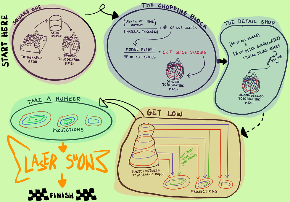
Algorithm Overview
The process begins when a user imports a topographic model as a polysurface or Brep. For my project I used a remixed model of the Matterhorn by "lastloginnname" on Thingiverse (linked here). The model is then trimmed into a circular shape for visual appeal. The user can adjust the diameter of this circular cutout to control how much of the topography is included in the final piece.
Next, the user sets two key parameters: the desired final height of the assembled model (after all layers are stacked) and the thickness of the material being used. These settings determine the number of slices that will be generated. If the material is thick relative to the model’s height, fewer slices will be produced, resulting in a lower-resolution output. To address this, I included an optional "detail layers" feature. This allows users to specify how many etched contour lines they want on each slice’s surface, mimicking the stylization of topographic maps and enhancing visual detail, even with fewer physical layers.
To support accurate assembly, each slice is etched with its layer number. Additionally, the outline of the next layer is engraved onto the current one. This means users can simply align each new slice with the outline beneath it, making the assembly process more intuitive.
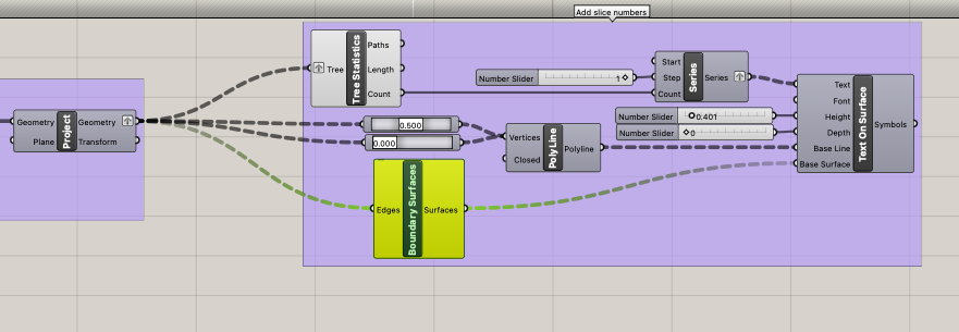
Screenshot of Grasshopper Code (click here to view and download full grasshopper script on GitHub)


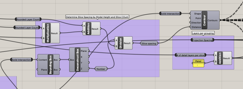


Visual Summary of Code Functionality
Parameters and Outputs
Parameters | Intermediate Outputs | Final Outputs |
Final output thickness | Number of slices | Slices spread on 2D plain |
Material thickness | Z Distance between slices | including detail etches |
# of detail etches/slice | Sliced Object | including past slice outline |
Topographic polysurface | including layer numbers | |
Projection spacing | ||
Diameter of trimming cylinder |
Key Algorithms
I used a previous slicer I built (see blog post "Stacking Up") as the foundation for this project, so the algorithm for generating the slices themselves was not novel for this project. The primary computational challenge I faced for this project was laying out the etched layers, sliced outlines, and etched outlines of the next layer in the correct groupings with consideration to the dynamic nature of the algorithm's parameters. In order to address the issue of proper laying out and grouping of slices I created three separate algorithms.

Algorithm to Project the Cutting Slices
I first needed a way to separate out which slices were outlines of layers that would be sliced. Sliced layers, which need to be treated distinctly from the detail etches generated despite being in the same tree, occur every # of detail layers + 1. I therefore was able to parse which layers were outline layers by taking the modulus of the number of total layers and the calculated sliced layer interval. Any modulus that equaled zero, that is to say was evenly divisible, occurred at a sliced layer interval and therefore was an outline of a slice. I took only those identified slices and arrayed them by multiplying their order in the series (ex. the second slice is 1) by the projection spacing parameter (ex. 19) to determine the distance the slice would move (ex. 1x19 = 19mm). Finally I projected those moved slices on to the XY plane, as they had a Z-value. When I baked these cutting slice outlines, I baked them onto their own layer so that I could set that layer to slicing, which all other outputs would be baked into a different layer for etching.
Algorithm to Project the Previous Layer Outline
In order to etch an outline of the next layer onto each cut slice as an orientation guide for assembly, I followed the same procedure as I did to project the cutting slices. The key different for this algorithm was that I used the Cull Index function to remove the first slice outline, as there is no layer below it to etch onto. This reordered the index so that each layer outline was one place below its match in the cutting slice index. The second slice in the cutting algorithm became the first slice in this algorithm, changing its movement in the array function to match that of the layer below it. This means the outline projected on the to cut layer one step below the cut layer it represented, creating a guide on the lower layer. It was in this layer projection that I added text onto each layer to identify the layer number of each cutting, as it was the innermost line and would be covered by the stacking of the next layer in assembly.
Algorithm to Project Detail Layers
The final feature I needed to add to my projected slices was the detail etches for each layer. This required grouping each set of etches onto the nearest cutting layer below it. In order to achieve this I used the series count variable and used integer division on it with the previously calculated sliced layer interval (# of detail layers + 1). This grouped the contours into sets of the outer cutting layer and its associated detail layers. I them multiplied the integer division results by the projection spacing to match the projections the two other algorithms created.
Fabrication

Parameters Used in each Model Generated
Model 1 | Model 2 | Model 3 | Model 4 | |
|---|---|---|---|---|
Final Depth | 2 mm | 24 mm | 10 mm | 18 mm |
Material Thickness | 2 mm | 2 mm | 2 mm | 0.25 mm |
Detail Layers per Slice | 8 | 2 | 2 | 0 |
Cylinder Trim Size | 15 mm | 15 mm | 15 mm | 15 mm |
Spacing Between Projections | 32 mm | 32 mm | 32 mm | 32 mm |
Laser Cutting Process
Once I had all of my slices produced and moved properly, I baked every etched slice into one layer and the slices for cutting into another. This allowed me to easily differentiate the settings for cutting and etching when communicating with the laser cutter.
For my fabrication I created Model 1, Model 2, and Model 3 from a dense 2mm cardboard and Model 4 from 0.25mm thick cardstock paper. I created rectangles in Rhino representing the dimensions of these sheets of materials and moved each layer onto a sheet of material to make cutting as efficient as possible. I combined the slices for Models 1-3 onto shared sheets and created three sheets for only Model 4, as it has nearly 80 slices and was a different material.
I began with slicing the first three models out of the dense cardboard. I had some trouble with this as the laser continually failed to cut all the way through the smoother edges of the circles. It had no trouble cutting through the rougher detailed edges. After many setting adjustments I resorted to breaking the circular pieces out of the cardboard along the partially cut lines and cleaning them up with scissors.

Assembly Process
Once I had each piece it was time to assemble the layers. This process was relatively simple: glue each piece to the piece below it within the marked outline, stacking by increasing layer number. Model 1 required no assembly , as its parameters made it a 2D only model.

The assembly of Model 4, which had over 70 layers, was made easier by the way I laser cut it, perforating the outlines enough that they could easily pop out, but so that they reminded in place until intentionally removed. This way I did not have to keep track of every layer at once, only the one I had just popped out. I applied glue to the back of each layer before popping it out for the cleanest possible application. One feature of Model 4 is that the laser cutter slightly browned the edge of each piece as it cut it, creating a really interesting effect and making the mountain look even more realistic from the side.


Reflection
Overall, this project turned out how I had hoped. I was able to create interesting sliced topographic models by using both 2D and 3D displays concurrently, resulting in a detailed and interesting output. One unexpected challenge was finding a usable topographical model. I had originally hoped to work with a large area, such as the entire state of Colorado or a mountain range. However, I ran into issues because these models are typically generated as meshes, and cutting a circular shape out of a mesh is very difficult. As a result, I was limited to meshes that I could convert into polysurfaces in Rhino, a process that requires significant computing power. Even then, some topographies were so complex that my computer couldn’t handle slicing them. Ultimately, I had to use smaller, less complex models for my final output.
Another issue I encountered involved the detail etch layers. In my model, the outline of each cut layer was included in the etch, which meant the laser would trace the outline before cutting. While this didn’t affect the final output, it did waste time during fabrication. To work around this, I manually deleted the etched outlines after baking the projections into Rhino. If I had more time, I would refine my detail etch algorithm to exclude the outlines automatically, streamlining the process and saving time.
While my project may not be as ambitious as Christopher Warren's Elk Mountain sculpture, I’m pleased with what I achieved in just a few weeks. The final output has the fidelity and features I was aiming for. I believe this slicer has real potential for creative applications that go beyond the current use case. For example, it would be fascinating to create a large installation of inverse slices, which would create "slices of the sky," so that someone walking through a room could feel as though they were inside a mountain. On the smaller scale, the slicer could be used to make objects like coasters by producing a clean circular top cutout with a standard-height rim, showcasing the mountain topography inside. The creative possibilities with this tool are extensive.


Comments